Every evening, someone has to put a number on thousands of bonds that nobody traded that day. Fund administrators need it to strike a NAV. Risk teams need it for limits, collateral desks for margin calls, auditors for year-end marks. The number has to be defensible even when the last real trade is weeks old.
The gap is large. On a typical day in 2025, about 14,600 US corporate bonds had traded at least once in the previous year. Only 54% of them traded that day, and almost a quarter had not traded for more than a month.
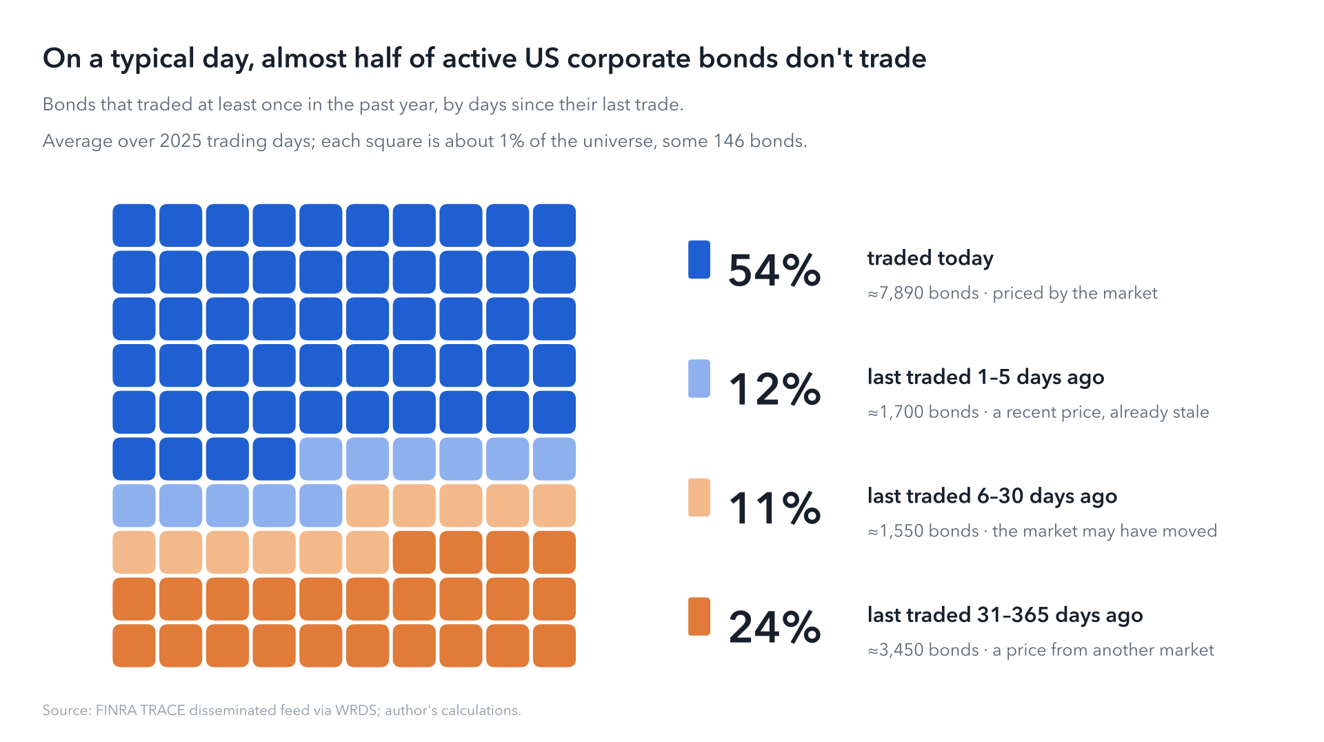
I built a model for that gap: a transformer that reads the whole day's market at once and prices the bonds that didn't trade, much as a trader scans the screen before marking a book. On 107 trading days of 2026 it had never seen, it beat every method I tested. It also says how sure it is, and those ranges hold up.
In short
- Its error was 7.4% lower than a LightGBM model with 79 features, and 11% lower than the last trade plus the day's market move.
- It was more accurate than LightGBM on 101 of the 107 days, and in every month.
- On bonds untraded for more than a month, it was 21% more accurate than the simple rule.
- Its 90% ranges held 91% of realized spreads: narrow where pricing is easy, wide where it is hard.
The bar is higher than it looks
The obvious approach is surprisingly hard to beat. Take a bond's last trade and carry it forward with the index of its rating bucket. Then add today's median move among similar bonds that did trade, in the same rating and maturity bucket. I call this carry plus move. In the first half of 2026 it missed realized spreads by just 4.55 basis points on average.
A well-built machine-learning model does better. My strongest baseline is a LightGBM model that predicts what carry plus move gets wrong, from 79 features: ratings, terms, liquidity measures, trading history, the day's market, and how the issuer's other bonds traded that day. It learned from the same years, under the same scenarios, and gets to 4.37 bp.
So the real test is to beat both, on the same bonds, day after day, by more than noise. That is the standard I held the model to.
The idea: let the model read the market
When a trader marks a bond that didn't trade, they look at what did: the issuer's other bonds, close comparables, the day's moves in the same part of the curve. Then they adjust from the last print.
The model does the same thing, at scale. Each trading day becomes a table. Some rows are bonds that traded, with their spreads. Others are bonds to price, with their spreads hidden. A transformer reads the whole table at once and returns a full distribution for every hidden bond.
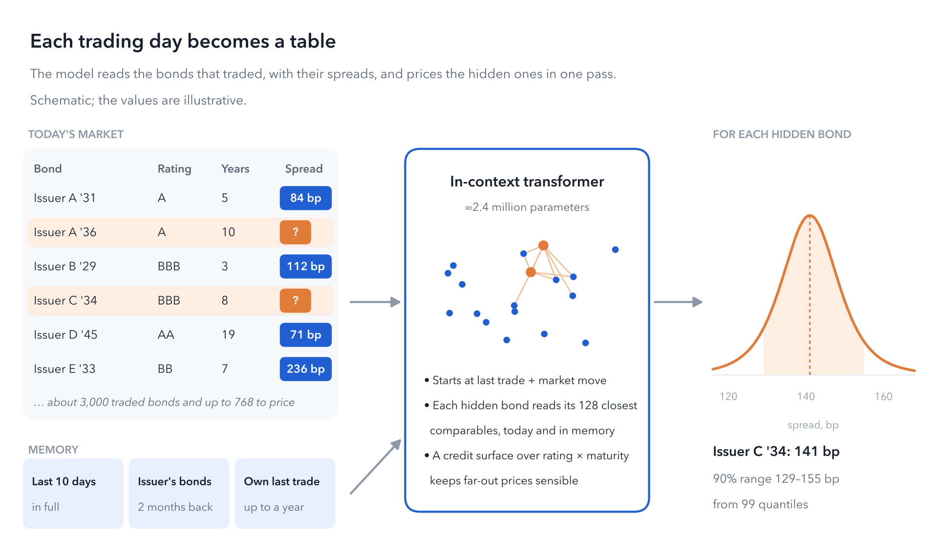
This is in-context learning, the idea behind tabular foundation models such as [TabPFN](https://www.nature.com/articles/s41586-024-08328-6) and [TabICL](https://arxiv.org/abs/2502.05564). The model doesn't learn which bond is which. It learns how to price from a day's evidence, so it adapts to each day's market without retraining.
Each row carries what a credit analyst would look at: rating, coupon, maturity, call features, seniority, sector, size and age; how often and how cheaply the bond trades; its last trade and how old that is; and the day's market, from Treasury yields to VIX and credit indices.
Six design choices that matter
It starts from the simple rule. Carry plus move is computed inside the model, and every correction starts at zero. Before any training the model is the baseline, and everything it learns is an improvement on top. That keeps it anchored on quiet days and makes its behavior easy to audit.
It can't memorize bonds. Issuers enter as random codes, reshuffled every day. The model can tell that two bonds share an issuer today, but it can never recall an issuer across years. It has to reason from evidence, which is what lets it carry over to bonds and days it has never seen.
It reads comparables across days. Each hidden bond attends to its 128 closest peers, today and in memory: same issuer, same sector, nearby on the curve, recently traded.
It keeps a credit surface. A spread surface over rating and maturity, constrained to widen as ratings fall, gives a sensible reference where comparables are thin, such as a long bond from a rarely traded issuer.
It remembers selectively. It reads the last ten trading days in full, the issuer's bonds two months back, and each bond's own last trade, up to a year old, next to the issuer's other bonds on that day. That last piece lets it compare the issuer's curve then with the curve now.
It reports a distribution, not a point. It outputs 99 quantiles per bond, so every price comes with a range.
It is also small: about 2.4 million parameters, trained on 19 years of data in about 1 hour on a single cloud GPU. A full day of the US market prices in seconds on a laptop.
Testing it the way it would be used
A pricing model is only as good as its test.
Time. The model trained on about 4,700 trading days from 2005 to 2023, and 2024–2025 picked the checkpoint. The test runs from 2 January to 5 June 2026: 107 trading days used for neither.
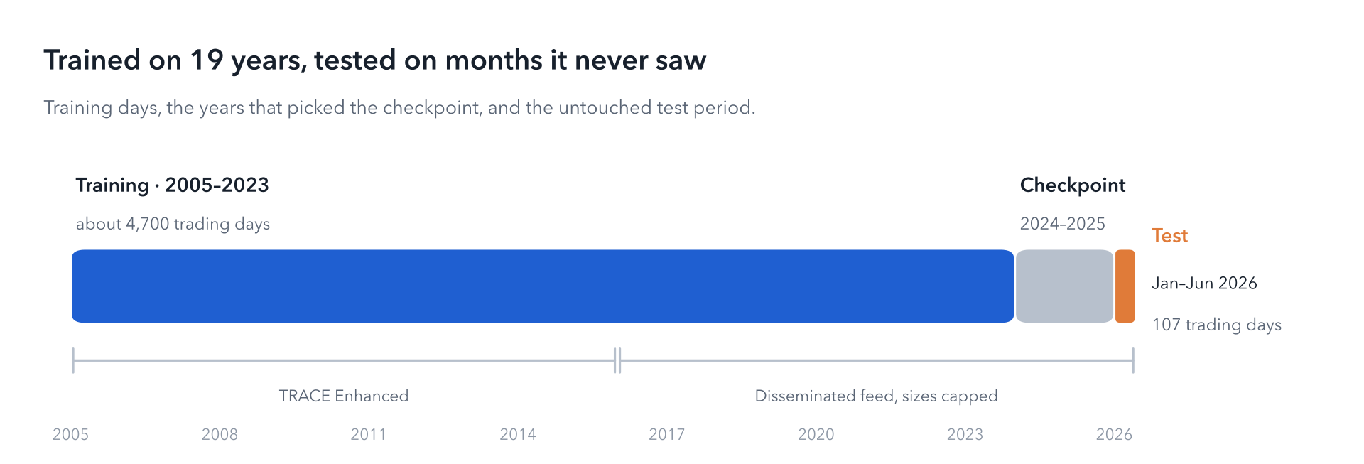
The data a live desk sees. From 2016 the prices come from the disseminated TRACE feed, the one a live system receives, with large trade sizes capped. Earlier years use TRACE Enhanced.
Realistic gaps. Each test day hides bonds in one of five ways, and a separate test hides every stale bond at once.
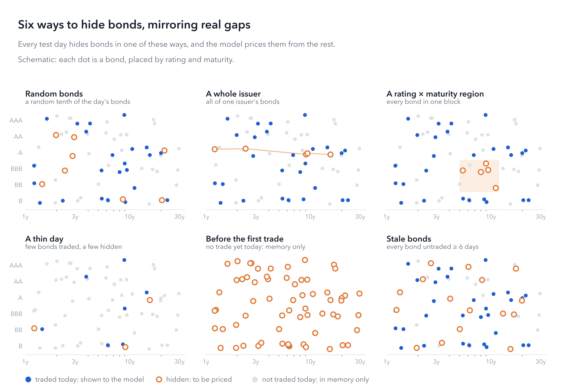
Every method priced exactly the same hidden bonds from the same information. I compare the average absolute error in basis points of spread. Differences are tested with Diebold–Mariano tests on daily errors and with a bootstrap that resamples whole days, since errors on the same day move together.
Results
Lowest error in both tests
Across the five daily scenarios, the transformer's average error was 4.05 bp, against 4.37 for LightGBM and 4.55 for carry plus move. In the stale-bond test, where all 31,587 bonds untraded for six days or more were hidden at once, it was 12.68 bp against 13.42 and 14.75.
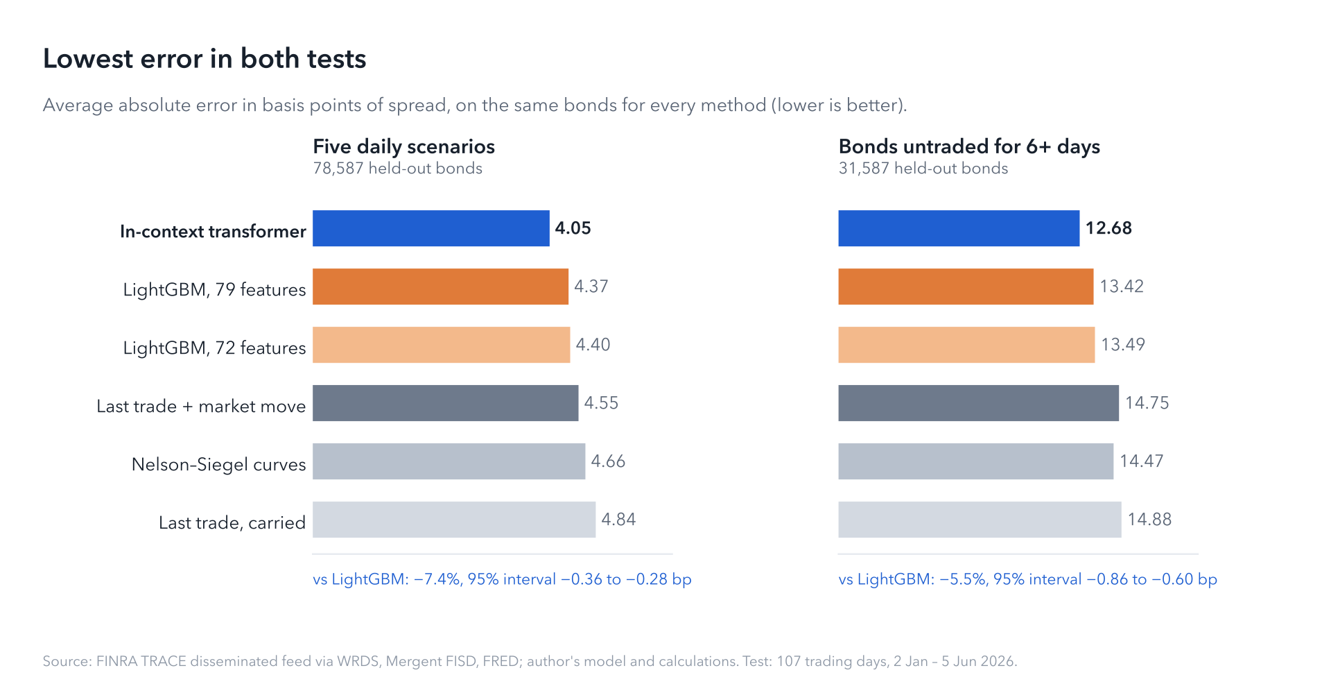
The gap to LightGBM is 0.32 bp in the daily scenarios (95% interval 0.28 to 0.36 bp) and 0.73 bp on stale bonds (0.60 to 0.86 bp). Neither is noise: the Diebold–Mariano t-statistics are −5.9 and −6.7. Against carry plus move, the error is 11% lower.
Not a lucky stretch
An average can hide a few lucky days. The transformer had the lower error on 101 of the 107 test days, and in each of the six months, including the volatile weeks of March and April.
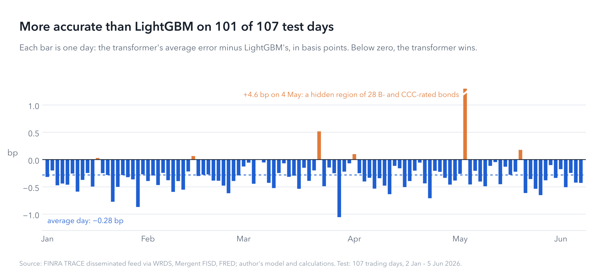
The one large miss tells its own story. On 4 May the hidden bonds were a whole region of 28 B- and CCC-rated bonds. The model applied the day's market move to them, and those distressed names didn't follow it. LightGBM, which discounted the move, did better. It is the clearest sign of where the model is weakest, and I come back to it below.
Stale bonds: where simple rules break down
Pricing a bond that traded yesterday is relatively easy. The hard case is the bond that last traded weeks or months ago. The longer a bond goes quiet, the more carry plus move drifts: its error climbs from 10.9 bp for bonds 6–10 days stale to 24 bp after a month, and 31 bp after four. The transformer's error rises much more slowly.
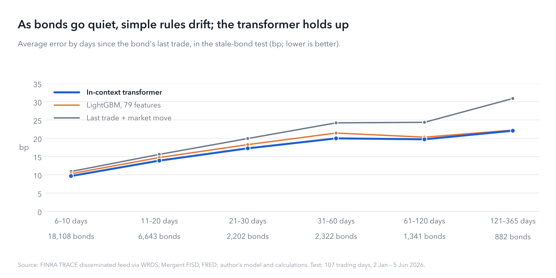
For bonds untraded for more than a month, its error was 21% below carry plus move (20.7 bp against 26.2) and 3.8% below LightGBM (21.5), with less bias: −3 bp against −7 for LightGBM. Beyond four months, the two models converge.
Where the gains come from
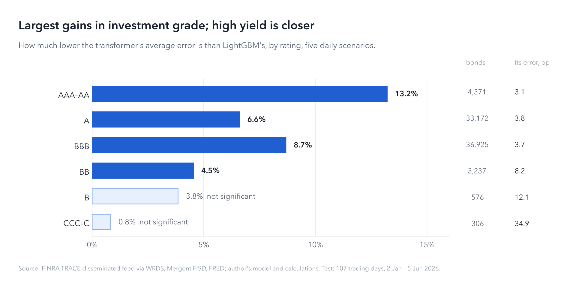
The edge is largest in investment grade, the bulk of the market: 13% lower error than LightGBM for AAA–AA bonds, 9% for BBB and 7% for A. It narrows in high yield, to 4.5% for BB and a statistical tie for B and CCC.
Every daily scenario shows the same pattern. With a whole issuer hidden, the transformer's error was 3.97 bp against 4.38 for LightGBM. On thin days it was 4.18 against 4.51. Before the day's first trade, with no trades from that day at all, it was 4.38 against 4.71.
It also reads direction better. When a spread had moved more than 1 bp since the bond's last trade, the transformer called the direction right 75% of the time, against 71% for LightGBM.
Uncertainty you can act on
A price is more useful with an honest range, and the model's ranges are calibrated at every level. Its 50%, 80%, 90% and 95% ranges held 51%, 81%, 91% and 95% of realized spreads. For stale bonds the figures were 49%, 79%, 90% and 95%.
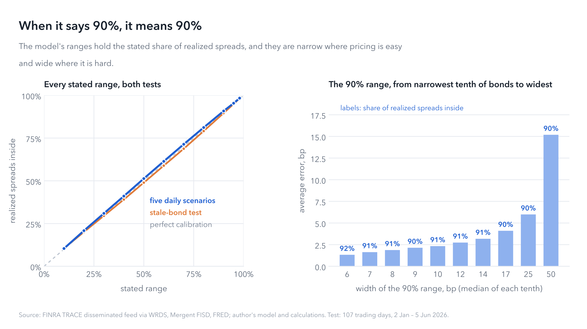
The ranges are also sharp. They are narrow where pricing is easy, about 6 bp wide for the most predictable tenth of bonds, and wide where it is hard, about 50 bp for the least predictable tenth. In every tenth, they held about 90% of outcomes. LightGBM's ranges, built from its past errors by rating and staleness, held 95% of outcomes but were much wider. On the continuous ranked probability score, which rewards ranges that are both calibrated and tight, the transformer scored 2.95 bp against 3.58 for LightGBM.
What it is worth
In price terms, the transformer's average error was $1,945 per $1 million of bonds per bond-day, against $2,092 for LightGBM and $2,151 for carry plus move. That is $150 to $200 less, for every bond, every day. On stale bonds the figures are $6,820, $7,082 and $7,861. For investment-grade bonds the average price error is 0.19 points per 100 of face value.
Where it still struggles
- Distressed credit. For CCC bonds the plain last trade is as good as anything: 33.8 bp against the transformer's 34.9, on 306 bonds. The market move the model starts from doesn't fit names that trade on their own news, as the 4 May region showed.
- Single-B bonds. On 576 B-rated bonds, the transformer and LightGBM are statistically tied.
- New issues. For 127 bonds with no earlier trade, most of them on their first day of trading, errors were around 25 bp, and long maturities were priced too wide.
Why this matters
Most of the corporate bond market is priced, most days, without a trade. A model that reads the market the way a trader does, says how sure it is, and can show the comparables behind each price fits several jobs:
- End-of-day marks and independent price verification, as a challenger next to an existing price source, with its edge measured bond by bond.
- Bonds that have gone quiet, where simple rules drift the most.
- Flagging off-market prints, quotes and marks. A calibrated range separates an unusual price from one that merely differs from a model.
- Pre-trade checks. You can see where a dealer's quote sits inside the model's distribution before the trade.
And because it is cheap to run, pricing the whole universe every evening is practical.
What's next: liquidity within comparable bonds
Every spread mixes two things: credit risk and liquidity. A bond can look cheap because the issuer is riskier, or simply because it is hard to trade, and the two call for very different decisions.
Today the model's credit surface runs over rating and maturity, so liquidity is folded into it. The next step adds a second surface, over each bond's illiquidity rank among comparable bonds of the same rating and sector, constrained so that spreads can only rise as liquidity worsens. Each price then splits into a credit part and a liquidity premium relative to its peers.
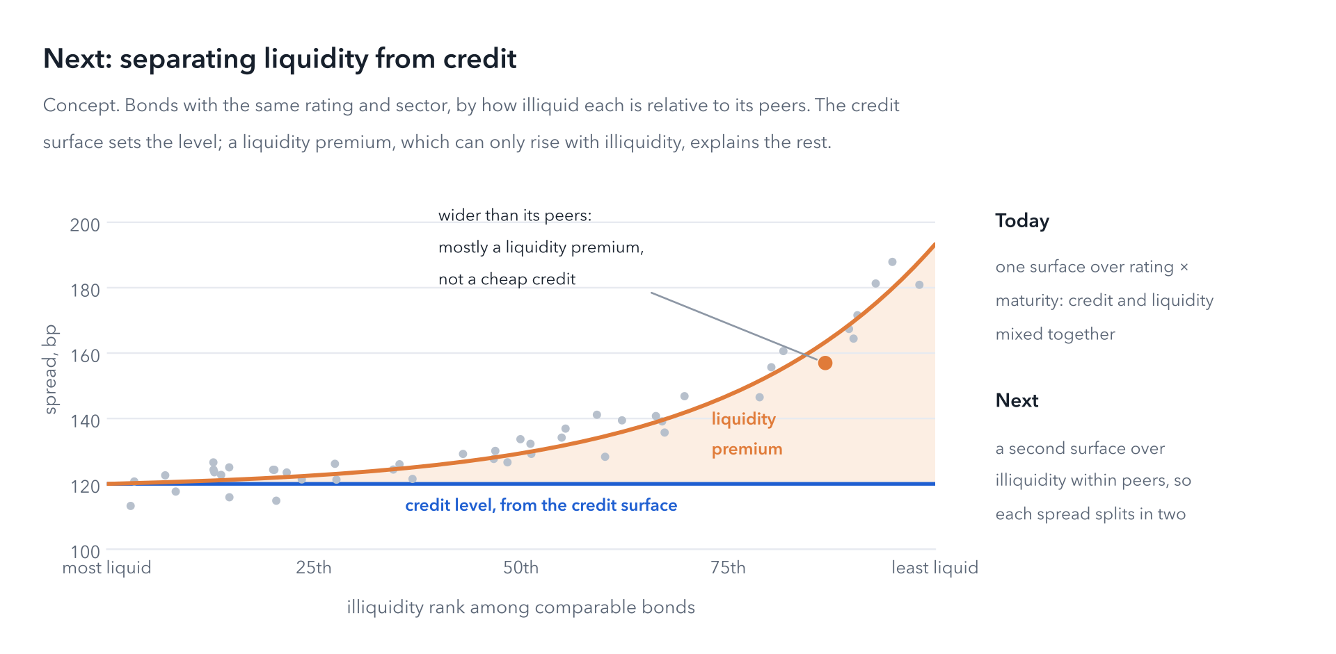
That split is what a portfolio manager needs before calling a bond cheap. A risk manager needs it too, to know how much of a mark rests on a bond being hard to sell.
If you price bonds that don't trade every day, I'd love to compare notes.
Notes on method
Data. US corporate bond trades come from FINRA TRACE via WRDS: TRACE Enhanced for 2005–2015, and from 2016 the disseminated feed that a live system receives, as cleaned by WRDS, with trade sizes capped at $5 million for investment grade and $1 million for high yield. Bond terms and ratings come from Mergent FISD, and market data (Treasury yields, VIX, high-yield and Baa spreads) from FRED. Each bond has one spread per trading day.
Scenarios. Each test day uses one of five scenarios, in roughly equal numbers: random bonds, a whole issuer, a rating-by-maturity region, a thin day, or a nowcast with no same-day trades. The separate stale-bond test hides every bond last traded six or more days before. Bonds without any earlier trade are reported separately, since most baselines need a last trade.
Baselines.
- Last trade, carried by its rating bucket's index.
- Carry plus the day's median move in the bond's rating and maturity bucket.
- Nelson–Siegel curves per rating bucket, plus each bond's own offset.
- Two LightGBM models of the carry-plus-move residual. They were trained on every fourth training day, about 800,000 hidden bonds over 1,186 days, under the same scenarios. The stacked version adds issuer-curve and Nelson–Siegel signals and the issuer's same-day news.
The baselines' ranges come from their residuals on training years, by rating and staleness.
Statistics. Diebold–Mariano tests use daily mean absolute errors with a Newey–West variance. The 95% intervals come from a bootstrap over days. Price errors convert spread errors with each bond's spread duration and price.
The model. About 2.4 million parameters: a row encoder, then four in-context attention layers 128 units wide. It outputs 99 quantiles per bond. It made 25 passes over the training years, and the checkpoint was chosen on 2024–2025. Predictions are averaged over four draws of the memory.
Detailed results, on the same bonds for every method (errors in basis points of spread):
References
- Hollmann, N., Müller, S., Purucker, L., et al. (2025). [Accurate predictions on small data with a tabular foundation model](https://www.nature.com/articles/s41586-024-08328-6). Nature 637, 319–326.
- Qu, J., Holzmüller, D., Varoquaux, G., and Le Morvan, M. (2025). [TabICL: A tabular foundation model for in-context learning on large data](https://arxiv.org/abs/2502.05564). ICML 2025.
- Ke, G., et al. (2017). LightGBM: A highly efficient gradient boosting decision tree. NeurIPS 2017.
- Nelson, C. R., and Siegel, A. F. (1987). Parsimonious modeling of yield curves. Journal of Business 60(4), 473–489.
- Diebold, F. X., and Mariano, R. S. (1995). Comparing predictive accuracy. Journal of Business & Economic Statistics 13(3), 253–263.
- Gneiting, T., and Raftery, A. E. (2007). Strictly proper scoring rules, prediction, and estimation. Journal of the American Statistical Association 102(477), 359–378.